
Calculating Multiple Linear Regression Parameters
Linear regression is used to find a linear relationship between a target and one or more predictors. Multiple linear regression explains the relationship between one dependent variable (Y) and two or more independent variables ($X_1, X_2, X_3 … X_n$).
\[\hat{Y} = B_0 + B_1.X_1 + B_2.X_2+...+B_n.X_n - e\]- Y - is the orignal score
- $\hat{Y}$ - is the predicted score
- e - is the error (Y - $\hat{Y}$)
- $B_0$ - is the intercept also known as regression constant
- $B_n$ - is the slope also known as regression coefficient
- $X_n$ - are predictor variables
- n - is the number of predic variables.
With the growing data science community and open source projects. There are enough packages and libraries to help anyone from getting started to deploy Multiple Linear Regression models into production. These packages easily help us in computing coefficients.It will be a nice thought to learn how these coefficients are computed. In this blog we’ll see how some of the packages use Normal Equations to compute the parameters.
The process of derivation is more convenient with the help of vectors and matrices.
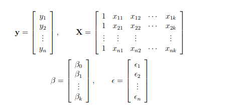
With this compact notation, the linear regression model can be written in the form.
\[Y = Xß + e\]We want to find the “best” β in the sense that the sum of squared residuals is minimized. The smallest possible value so that the sum of squares could be zero. If value of i reached zero, then.
\[\hat{Y} = X\hat{ß}\]The $\hat{Y}$ is the predicted values in our regression model that all lie on regression hyper-plane. Suppose further that betahat satisfies the above equation. Then residuals e(Y - $\hat{Y}$) are orthogonal (perpendicular) to the columns X (Input matrix) then
\[X^T(Y - X\hat{ß}) = 0\] \[X^TY - X^TX\hat{ß} = 0\] \[X^TX\hat{ß} = X^TY\]These vector normal equations are similar to normal equations that can be obtained using derivatives. To find the best fit estimated parameters for the $\hat{ß}$, We need to solve the normal equation so by multiplying both side by $X^TX$ we will get
\[\hat{ß} = (X^TX)^{-1} X^TY\]- $X^T$ - is known as X-transpose(switch rows with the columns of the matrix)
- $X^TX$ - is the dot product between X and X-Transpose
- $(X^TX)^{-1}$ - is the inverser of $X^TX$
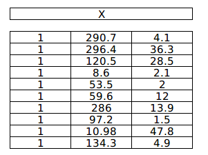
Let’s use this equation to find the best fit estimated parameters for our example. To solve this normal equation all you need to know is matrix addition, subtraction, matrix multiplication (Dot product) and Inverse. Please note that following computations are done for the purpose of understanding the process of estimating parameters.
Feature matrix X
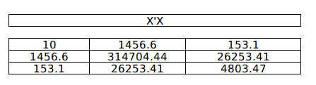
Dot product of X & $X^TX$
$(X^TX)^{-1}$
-1.png)
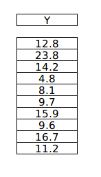
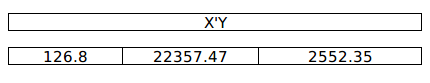
Y target variable vector
Dot product of $X^TX$ & Y
And finally $(X^TX)^{-1} X^TY$
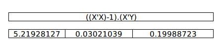
To verify our estimated values let us use sklearn package to see how close the values are to the package’s computed values.
from sklearn import linear_model
X = sample_df[[X1,'X2]]
Y = sample_df[‘Y']

regr = linear_model.LinearRegression()
regr.fit(X, Y)

print('Intercept: \n', regr.intercept_)
print('Coefficients: \n', regr.coef_)
Intercept: 5.219281272910356
Coefficients: [0.03021039 0.19988723]
The values are exactly the same, showing that sklearn’s linear_model uses Normal Equations to compute the coefficients.